If you search online for methods of calculating π, you’ll find countless ways. This is yet another one, probably complex, definitely imperfect, but at least you’ll learn more about the Monte Carlo methods.
The value of π
I’m pretty sure you’ve met π before. It should have been part of your school years, but I don’t expect you to have fond memories of it. It has been part of plenty of works of science fiction too, where one of my favorites is Carl Sagan’s Contact.
π is an endless sequence of digits, starting with 3.1415926535897932384626433832795. For those of us old enough to know what a slide rule is, it was right there, waiting to be used in calculations. In geometry, if you needed to straighten a circumference, you’d multiply the diameter by 22 and divide by 7; 22÷7 is 3.142… (far from π, but close enough given the limited resources). When electronic calculators became popular, one could use 355÷113 (3.14159292…; closer, but not yet perfect).
In theory, one should be able to determine π precisely through a simple division. If the length of a circumference is π times the diameter, then you could simply measure the circumference and the diameter, and then divide the former by the latter. Possibly a more precise calculation would be to divide the area of a circle by the square of the radius. Unfortunately, both methods fail because the precision of the result is limited to the precision of the measurements.
Or you could use a statistical method, couldn’t you?
Monte Carlo experiments
Monte Carlo methods (or experiments) are a set of algorithms that rely on repeated random sampling to obtain numerical results.1 In practical terms, you collect so many random numbers to see which ones conform to the rules you’re evaluating. If you’re still scratching your head, let’s jump to action!
Area of a circle: π×r²
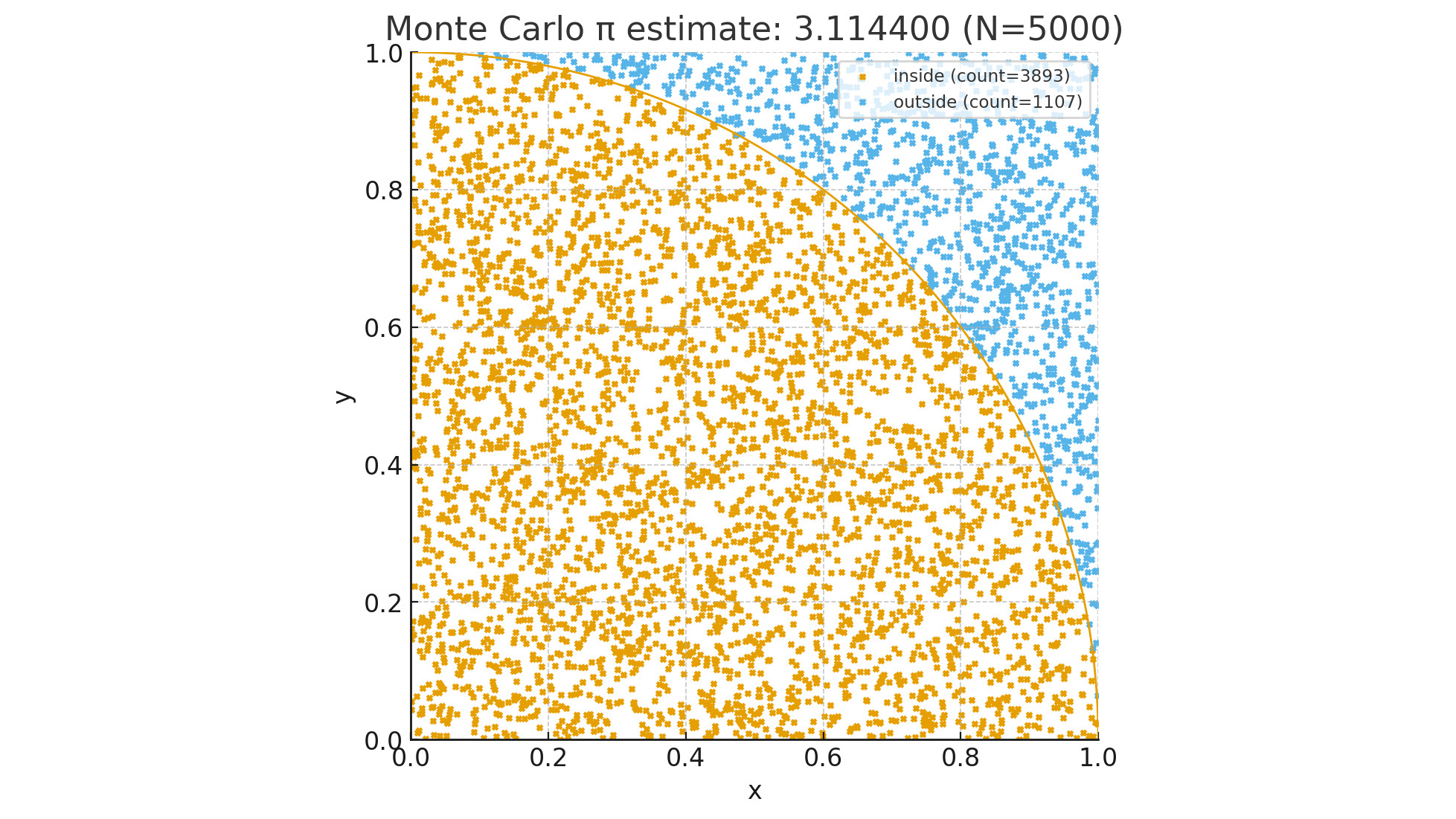
As mentioned earlier, you could determine π by dividing the area of a circle by the square of the radius. Assuming you have a circle inscribed in a square, that is, a circle enclosed in a square and intersecting all four sides, then you could start selecting random points inside the square and choose the ones inside the circle. If you then divide the number of points inside the circle by the total number of points, you’ll have a good approximation. Also, the more points you use, the more precise the result.
Let’s create a computer program for this simulation. To make matters easier, let’s set the radius to 1 (one squared is still one). To make it even easier, let’s use a quarter circle inside a quarter square, just like the picture at the top of this page. For this program to work, we’ll make it choose X and Y coordinates between 0 and 1 for each point. If the distance between the center of the circle and the point is 1 or less, then it’s inside the circle and outside otherwise.
Here’s the Python program:
import secrets
import sys


def get_random() -> float:
    return secrets.randbelow(1000) / 1000


def is_inside(x: float, y: float) -> bool:
    return x * x + y * y <= 1


n = 100_000_000 if len(sys.argv) == 1 else int(sys.argv[1])
inside = 0
for _ in range(n):
    if is_inside(get_random(), get_random()):
        inside += 1
print(inside * 4 / n)
We’re using secrets because it uses the computer random number generator, and we accept a command line argument with the number of points to use (default: 100 million). Because we’re using a quarter of a circle, we need to multiply the result by 4. A sample run on my computer gave me 3.14564084 but it took longer than a minute; I can’t wait that long! For the record, it’s a 13th generation Intel i9 with 20 cores at 5.4GHz; it’s a very powerful machine, but certainly not enough for this exercise.
Or is Python the problem? Python is incredibly powerful and easy to use, but for heavy calculations, it’s not necessarily the best choice. Let’s rewrite the program in Go:
package main

import (
	"fmt"
	"math/rand"
	"os"
	"strconv"
)

func main() {
	inside := 0
	n := 100_000_000
	if len(os.Args) > 1 {
		n, _ = strconv.Atoi(os.Args[1])
	}
	for range n {
		x := rand.Float64()
		y := rand.Float64()
		if x*x+y*y <= 1 {
			inside++
		}
	}
	fmt.Println(float64(inside) * 4 / float64(n))
}
How does it perform? On the same computer, it gave me 3.1415122 in less than a second and a half, and 3.1416738 on the second run. Depending on the version of Go you have, you could replace math/rand with math/rand/v2, which will cut your execution time even further; for example, it gave me 3.1416448 in a little over 1 second. If I wanted to use more points, therefore increasing the precision, I could use 1 billion points for example; one result was 3.141558076 and it took less than 11 seconds.
I don’t love this outcome…!
I really don’t. That was too much effort that didn’t bring me much closer to π than 22÷7. Going forward, if I want to use π, I could use math.pi on my Python programs or, if I really wanted precision, I could head over to ClickCalculators.com and get 1,000 digits.
At the least, I brought you the Monte Carlo experiments, which you might find valuable.
And it made me curious too: how would other programming languages perform?
Other languages and tools
Spoiler alert: the table at the end of this article shows how each alternative performed.
More Python
Random number generation is a complicated matter. It involves a series of calculations based on an initial value, usually referred to as “seed.” Because random numbers can be used in cryptography, if one could replicate the seed than all cryptography is dismantled. In my initial program I was using secrets because it relies on the operating system itself, which makes it more secure. The tradeoff is that secrets uses /dev/random, which is a special file, and reading from files incurs delays. Let’s rewrite the program to use random instead.
import sys
from random import random


def calculate(n: int) -> float:
    inside = 0
    for _ in range(n):
        x = random()
        y = random()
        if x * x + y * y <= 1.0:
            inside += 1
    return inside * 4 / n


if __name__ == "__main__":
    n = 100_000_000 if len(sys.argv) == 1 else int(sys.argv[1])
    print(calculate(n))
It must be noted that, instead of a minute and a half, it took slightly over 10 seconds.
One characteristic of Python is that each program runs on a single CPU core. No matter how many cores you have, the program will only use one. For enterprise applications, this makes it beneficial because it’s easy to scale, but for calculation-intensive applications you’re not leveraging the full power of your computer. There are tools and mechanisms to spread your program execution across multiple cores, but it usually involves a major rewrite of your program.
Another characteristic of Python is that the program is converted to bytecode and interpreted at runtime. Depending on the case, this incurs slower execution time and increased resource usage. Specifically for numeric calculations, Numba could be your friend. Its first trick is to pre-compile the code so it doesn’t have to be interpreted at runtime. All it takes is a single @njit decorator and obviously importing the Numba library.
import sys
from random import random

from numba import njit


@njit
def calculate(n: int) -> float:
    inside = 0
    for _ in range(n):
        x = random()
        y = random()
        if x * x + y * y <= 1.0:
            inside += 1
    return inside * 4 / n


if __name__ == "__main__":
    n = 100_000_000 if len(sys.argv) == 1 else int(sys.argv[1])
    print(calculate(n))
Impressively enough, it ran in less than 3 seconds (considerably faster).
Another benefit is that Numba can spread NumPy array expressions across multiple CPU cores, which could speed it up. It’s all a matter of adding @njit(parallel=True).
Python 3.14
When I wrote the original article, I was using Python 3.13, but now I’ve upgraded to 3.14 and updated all timings. I also added rows to the table down below to differentiate between versions. You’ll notice that Python 3.14 with the secrets library ran considerably faster, while using random and numba performed a tad slower.
Mojo
Mojo is a relatively new language. For example, I’m currently using version 0.26.1.0, which is the latest on Arch Linux. The standard library is open source, but the compiler not yet. Its syntax is similar to Python and programs can be compiled to run on any hardware, including GPUs. As for the program, I could have used the very same source code, but instead I opted for a Mojo optimization:
import random
from sys import argv

fn main() raises -> None:
    n = 100_000_000 if len(argv()) == 1 else Int(argv()[1])
    random.seed()
    inside = 0
    for _ in range(n):
        x = random.random_float64()
        y = random.random_float64()
        if x*x + y*y <= 1:
            inside += 1
    print(inside * 4 / n)
The optimization is to use fn instead of def, which instructs the compiler to use Mojo mode. The other changes are just to comply with the Mojo syntax.
How did it perform? Much better than pure Python, but Numba is still giving Python an edge. If I had a GPU I could report better numbers, but I don’t have one, ergo I can’t. Perhaps you can?
OCaml
Out of pure curiosity, I’ve been studying OCaml recently. In case you’ve never heard of it, it’s geared towards functional programming, but it also allows for imperative programming. I’m using this double nature to measure its performance.
I’m not bothering exploring command line arguments and am hard coding 100 million iterations. The first example follows an imperative approach, which is more palatable for so many programmers.
let calculate number =
  let inside = ref 0 in
  for _ = 1 to number do
    let x = Random.float 1.0 in
    let y = Random.float 1.0 in
    if x *. x +. y *. y <= 1.0 then
      incr inside
  done;
  (float_of_int !inside /. float_of_int number) *. 4.0

let () =
  Random.self_init ();
  let number = 100_000_000 in
  let pi = calculate number in
  Printf.printf "%f\n" pi
The next example follows a functional approach to appease the purists and myself.
let calculate number =
  let rec loop i inside =
  if i >= number then
    (float_of_int inside /. float_of_int number) *. 4.0
  else
    let x = Random.float 1.0 in
    let y = Random.float 1.0 in
    let inside =
      if x *. x +. y *. y <= 1.0 then
        inside + 1
      else
        inside
    in
    loop (i + 1) inside
  in
  loop 0 0

let () =
  Random.self_init ();
  let number = 100_000_000 in
  let pi = calculate number in
  Printf.printf "%f\n" pi
This is very subjective (I know), but in my humble opinion, OCaml is a very beautiful language. Sadly, it only fits a very specific niche, mostly academic.
Please see the results down below.
Julia
In another article I talk about Julia in more detail, but in short, it’s a dynamic multi-paradigm general-purpose programming language with some pretty cool features geared toward engineering and data science. Here’s the program I’m using for the same:
is_inside(x ::Float64, y ::Float64) = x*x + y*y <= 1.0

function calculate(iterations ::Int)
    inside = 1
    for i in 1:iterations
        if is_inside(rand(), rand())
            inside += 1
        end
    end
    return inside * 4.0 / iterations
end

print(calculate(100_000_000))
Much to my surprise, or perhaps not at all, it’s the first one to consistently perform in less than one second.
Elixir
Elixir is a functional, concurrent, high-level general-purpose programming language created by my fellow Brazilian José Valim in 2012 that runs on the BEAM virtual machine, which is also used to implement the Erlang programming language. Elixir builds on top of Erlang and shares the same abstractions for building distributed, fault-tolerant applications. Elixir also provides tooling and an extensible design. The latter is supported by compile-time metaprogramming with macros and polymorphism via protocols.
defmodule Montecarlo do
  def pi(iterations) do
    calculate(iterations, 0) * 4 / iterations
  end

  defp calculate(count, sum) do
    if count == 0 do
      sum
    else
      x = :rand.uniform()
      y = :rand.uniform()
      inside = if x * x + y * y <= 1.0, do: 1, else: 0
      calculate(count - 1, sum + inside)
    end
  end
end

defmodule Montecarlo.CLI do
  def main(args \\ []) do
    args |> parse() |> Montecarlo.pi() |> IO.puts()
  end

  defp parse(args) do
    try do
      args |> hd |> String.to_integer()
    rescue
      _ in ArgumentError ->
        100_000_000
    end
  end
end
The major difficulty, when learning a new programming language, is not the learning itself, but to start thinking in terms of the language. For instance, imperative languages have a for statement that allows you, among other things, to iterate over a list. Functional languages do not. You can use recursion, like above.
Elixir provides plenty of tools for iterating over a list. The Enum module is very rich. By leveraging some of its functions, the code can be made easier to read, just like below. And how did it perform? I’ll let the numbers speak for themselves.
defmodule Montecarlo do
  def pi(iterations) do
    inside =
      1..iterations
      |> Enum.map(fn _ -> random_point() end)
      |> Enum.count(fn {x, y} -> x * x + y * y <= 1.0 end)

    4.0 * inside / iterations
  end

  defp random_point(), do: {:rand.uniform(), :rand.uniform()}
end
Please feel free to see my repo for the full source code.
From a timing perspective, Elixir shares a disadvantage with Java (not included in this article): before the program can run, it must first launch its virtual machine and verify the code. Python works almost the same way, interpreting the pre-compiled code instead of launching a virtual machine. Just keep in mind that Elixir is not tailored for desktop applications (although it does run on desktops with BEAM installed); instead, it’s better for servers.
But I’m stubborn. The beauty of Elixir (and Erlang, for that matter) is that fault tolerance is implemented by BEAM, so you don’t have to worry about it in your application. The price is poorer performance. Pick your poison.
C
Let’s have a formal baseline!
#include <stdio.h>
#include <stdlib.h>
#include <time.h>

static double random_double() {
    return (double) rand() / (double) RAND_MAX;
}

static double calculate(long n) {
    long inside = 0;
    srand(time(NULL));
    for (long i = 0; i < n; i++) {
        double x = random_double();
        double y = random_double();
        if (x*x + y*y <= 1.0)
            inside++;
    }
    return (double) inside * 4 / n;
}

int main(const int argc, const char *argv[]) {
    long n = 100000000;
    if (argc > 1)
        n = atol(argv[1]);
    printf("%lf\n", calculate(n));
    return 0;
}
Before you check the table below, let me spoil the surprise: Go ran faster than C! Less than 10% faster, yet faster nonetheless.
Comparison
In alphabetical order, this is how the different languages and tools performed. I’m omitting the calculated value of π because, for this exercise, it has become irrelevant.
| Name | Iterations | Sample Duration (seconds) |
|---|---|---|
| C | 100M | 1.628 |
| Elixir iterative | 100M | 35.640 |
| Elixir recursive | 100M | 10.487 |
Go with math/rand |
100M | 1.479 |
Go with math/rand/v2 |
100M | 1.106 |
| Julia | 100M | 0.567 |
| Mojo | 100M | 3.878 |
| OCaml functional | 100M | 1.815 |
| OCaml imperative | 100M | 1.834 |
| Python 3.13 with Numba | 100M | 1.902 |
Python 3.13 with random |
100M | 9.265 |
Python 3.13 with secrets |
100M | 100.849 |
| Python 3.14 with Numba | 100M | 2.108 |
Python 3.14 with random |
100M | 10.542 |
Python 3.14 with secrets |
100M | 77.705 |
Ranting
This is not a comprehensive, all inclusive, thorough benchmark. Instead, it’s just a use case. An example. Nothing else.
Should it influence you when deciding what to use on your next major project? I’ll leave it at your discretion. Is it going to influence me? Not at all! There are several factors to be considered when choosing a programming language, where performance and resource consumption should be on the top of the list, with mainstream adoption as a close third. I’ve left Zig off the list because it’s not mature enough, at least for me, but included Mojo because there’s a parade of geeks pushing for its adoption and I wanted to see how it compares. I’m not impressed, to be honest, and Julia far exceeded my expectations.
I’ve heard that Object Oriented Programming is a waste of brain power. OOP advocates claim that data needs structure and deserves behavior. I believe the real value is not in inheritance, but in messaging, meaning how you interact with objects.
I’ve also heard that Functional Programming is another waste of brain power, mostly due to immutability and lack of loops. My response to that is: isn’t predictability and consistency worth the effort? For me, it’s not a waste of brain power, but an investment. I’d rather burn my neurons figuring out how to make it work instead of wondering why it suddenly stopped working.
Meanwhile, my preferences are still (in no particular order) Go (for speed), Elixir (for robustness), and Python (for flexibility).
But something tells me I might be adding Julia to my list in no time.
Revision history
- 2025-09-27: Original posting date.
- 2025-10-08: Speeding up Python; Mojo.
- 2026-02-16: Python 3.14; C; OCaml.
- 2026-02-20: Julia.
- 2026-03-19: Elixir.
- 2026-03-20: Elixir refactored.
References
-
Source: Wikipedia: Monte Carlo method ↩